In part 1 of this series, we discussed the rise of Large Language Models (LLMs) such as GPT-4 from OpenAI and the challenges associated with building applications powered by LLMs and LLM deployment. Today, we will focus on the deployment challenges that come up when users want to accomplish LLM deployment within their own environment. We’ll explore the different techniques to overcome these challenges and make the deployment process smoother.
While customers can use GPT-4 or similar models to integrate into their applications, it is not always viable for users to depend on third-party endpoints to power their LLM applications. This is because users might have security and privacy concerns sending data to a 3rd party. Additionally, the OpenAI model might not be optimized for their specific use case, both in terms of model performance and deployment strategies.
Alternatively, users now have a wide variety of open source models (e.g. Llama2 and Falcon) that are edging closer to the performance of state-of-the-art closed source counterparts. This allows users to finetune models based on relevant data for the task and optimize the deployment for the specific requirements of their applications.
LLM Inference Challenges:
LLMs have unique characteristics when it comes to inference compared to other types of ML models.
A. Sequential Token Generation
LLM inference is autoregressive by nature. In other words, the current token generation consumes results from the previous generation. This serial execution order until completion typically has a high latency, especially if the task is generation heavy (i.e generating a lot of tokens for the result).
Moreover, given the variable length of the generation, it is not possible to know the expected latency before execution. For example, consider the task of answering a question “what is the capital of France.” The latency of serving this request is going to be fundamentally different from a document summarisation task. This poses scheduling challenges depending on the workload.
B. Variable Sized Input Prompts
As we discussed in the first part of this blog series, there are different prompt templates (zero vs few shot) that users could leverage to get better results from their LLMs. These prompting techniques have different lengths and therefore directly affect the amount of work required to process the input by the model. This is because the standard attention layer in the transformer architecture scales quadratically with the number of tokens in terms of compute and memory requirements. Batching requests with different prompts can also be challenging. One strategy is to add extra padding to match the longest prompt, but this isn’t very efficient from a computation point of view.
C. Low Batch Size
LLM inference payloads typically have a low batch size (which is different from training and finetuning). With low batch size, it is expected that the computation is bottlenecked on IO and would suffer from low GPU utilization. This is not ideal as users want to make the most out of their expensive GPU provisioning.
D. Attention Key-Value (KV) Cache
With autoregressive token generation, a common optimization is to keep a KV cache of previously generated tokens. This cache is used as input for the current token generation, helping to decrease unnecessary computation between steps. While this KV caching requirement optimizes computation, it has a larger memory footprint, which can become substantial when handling several simultaneous requests.
Based on the above characteristics of LLM inference, there are two main challenges that we will discuss further:
1) LLM Memory Requirement is a main bottleneck from deployment perspective, and it affects the choice of hardware that users need to provision.
2) Scheduling Strategies would enable a better user experience and optimal hardware utilization. The different configuration choices for optimization depend on the application.
For example, an interactive chat application requires a different setup from a document summarisation batch workload. If customers do not carefully choose the right setup, they are likely to end up either overprovisioning expensive GPU hardware or hurting the perceived latencies of end users.
In general we argue that optimizing LLM deployment is a multidimensional optimization challenge that is use case dependent.
LLM Memory Optimization:
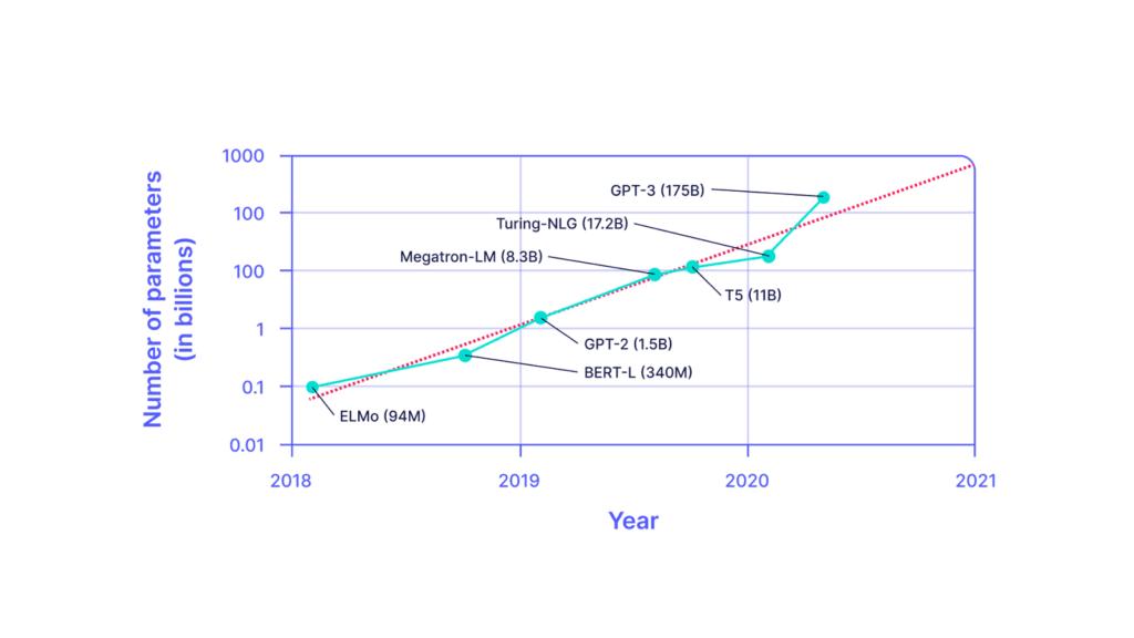
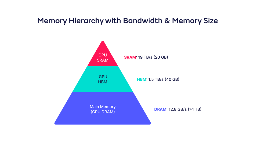
Current trends for LLMs are still pointing to larger models being better, as they have a larger capacity to learn with more parameters. GPT4 is likely to be in the trillion parameters range. It is unclear whether this trend is going to persist given that we are reaching the limits of training data. Nevertheless with a trillion parameters to load at inference time, this requires at least 2 TBs of GPU HBM (assuming fp16 precision).
In addition to loading model parameters, users have to account for memory related to the attention layers calculation and cache management. The push for in-context learning in LLM applications such as retrieval augmented generation (RAG) adds more pressure on the memory requirement.
Claude 2 allows for up to 100k tokens to be sent as an input prompt. Depending on the architecture, the memory requirement for a token in the KV cache can be in the order of 1 Megabyte. By extension, with many concurrent requests and big prompts, KV cache can easily get into the terabyte range.
However, memory capacity is not the only challenge. Users need to consider memory bandwidth as well. This is because a lot of data movement hurts performance, especially in the low batch size regime where typically the workload is IO bound.
There are various options that users could explore to get around such a memory bottleneck that we will explore next.
One approach to deploy LLMs that do not fit on one GPU is to employ some form of parallelism (e.g. sharding) across multiple GPUs.
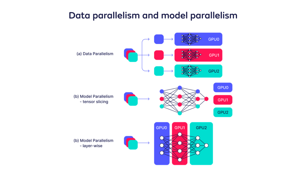
1. Data Parallelism (DP)
One technique of parallelism is DP. In this scenario we replicate the deployment of the model several times and split the incoming requests across the different replicas of the model. This allows the deployment to absorb a higher number of requests as they are served in parallel by the model replicas. However, if the model does not fit on a single GPU, then users need to leverage model parallelism.
2. Tensor Parallelism (TP)
One strategy for model parallelism is TP (intra-operation parallelism). In this case the model is split horizontally and each shard of the model resides on one GPU. In other words, each GPU is computing a partial result for a slice of the input tensor that corresponds to the slice of the weights that is loaded. The different shards are executed in parallel and at the end of one operation there is a synchronization step to combine the results before moving on to the next operation (layer).
Given that there is a lot of synchronization required for TP, it is recommended that the GPUs are colocated within the same node and interconnected with high-speed links (e.g. using NVLink).
3. Pipeline Parallelism (PP)
Another orthogonal approach that does not require a lot of synchronization among GPUs is PP (inter-operation parallelism). In PP the model is split vertically and each GPU hosts a set of layers. The GPUs form a pipeline, after one GPU is done computing the corresponding layers, the intermediate result is sent to the next GPU in the pipeline and so on. Although this strategy reduces the amount of synchronization and therefore can be used inter-node, PP is the simple setup that can suffer from low utilization as all but one GPU is idle (bubble).
There are techniques to get around this bubble by having different requests at different stages of the computation (i.e. computing on different GPUs) assuming that the traffic patterns allow for this strategy. This increases the overall throughput.
4. Hybrid Parallelism
The above techniques for parallelism can be combined together. For example one setup could be DP+TP in the case that the model cannot fit on one GPU (e.g. requiring at least 2 shards) and also replicated to serve a given inference load. With many configuration options, it is imperative that the parallelism setup is optimized according to the model, available hardware, traffic patterns and use case.
There are libraries that could be used to enable LLM model parallelism, such as deepspeed and parallelformers.
Compression (e.g. Quantization)
One strategy to reduce the memory requirement for LLMs is to use a form of compression. There are various techniques for compressing the model such as Distillation, Pruning and Quantisation. This blog post will focus on quantisation because it is a technique that can be applied at deployment time and does not require re-training of the model.
Quantisation reduces the memory footprint of the model by representing the model weights and activations with low-precision values e.g. by using int8 (1 byte) instead of fp32 (4 bytes). In this case the model requires 1 ⁄ 4 of memory compared to the unquantized version, which allows for deployments with less GPUs and therefore making it more affordable.
It is expected that Quantisation techniques have minimal effect on the model performance, however it is recommended to evaluate the quantised model depending on the use cases to make sure there is no substantial regression in the quality of the results.
When using mixed-precision quantisation, there are overheads associated with the quantisation process that could be noticeable (e.g. with medium sized models). Therefore this could result in sub-optimal inference latencies.
Possible libraries that could be leveraged for quantisation are bitsandbytes, gptq and deepspeed.
Attention Layer Optimization
Attention is at the heart of the transformer architecture. It has substantial memory and compute requirements, as standard attention scales quadratically with the number of tokens. This requires extra GPU memory capacity as intermediate (KV) results need to be cached. Additionally memory bandwidth is something that should be considered as these tensors are moved from GPU memory to the registers of the tensor cores.
There are techniques that help optimize the memory requirement for attention such as FlashAttention and PagedAttention. They typically help reduce the amount of data movement and therefore improve the latency and/or throughput of the attention layer.
However, these techniques are optimized for specific use cases such as low batch size and executing on a single GPU, and therefore should not be treated as a solution for every scenario.
Scheduling Optimization
As we described earlier, LLMs typically have high and variable latency at inference time. Therefore it is imperative that requests are scheduled efficiently on the model servers otherwise end users would complain about the usability of these LLM applications.
Scheduling can be done at different levels with corresponding tradeoffs that we are going to explore next.
Request Level Scheduling
A standard level of scheduling is at the granularity of a request. In this case when a request arrives at the model server, there is a decision whether to serve this request if there is compute space for it or add it to a pending requests queue to be served later. For example, assuming an idle server, if a request comes it will get served immediately as we have available compute capacity for it. If there are subsequent requests that arrive while the first request is being served, these requests will have to queue up until the first request is completely done.
Scheduling at the request level has some characteristics. If there is compute capacity available the request will be served as fast as possible. If we don’t address this, considering that serving a complete request with LLMs can take several seconds, other incoming requests would incur a high latency due to queueing delays until compute resources are available. Therefore unless there is a lot of compute replication it is likely that request level scheduling would suffer from high average latencies due to this head-of-line blocking issue. This also suffers from low GPU utilization as individual inference requests typically have low batch size.
Batch Level Scheduling
A way to build upon request-level scheduling is to batch requests within a timeframe and treat them as a single batch for scheduling. This is sometimes called adaptive batching. The benefits of this technique are:
1) It allows multiple requests to be served at the same time, which reduces the overall average latencies compared to request level scheduling
2) It increases the GPU utilization as the GPU is computing on a batch
However from a scheduling perspective, this batch of requests is static. In other words, if new requests arrive after a batch is formed, these new requests have to queue up until this batch is done. So, the time it takes to process a batch is determined by the longest generation request in that batch. This can unnecessarily delay other requests from being served.
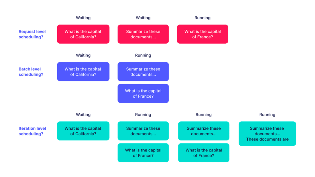
Iteration Level Scheduling and Continuous Batching
The techniques mentioned above have a downside: incoming requests have to wait in the queue until the ongoing generation finishes. This causes unnecessary delays and increases latencies.
The solution around this issue is to dynamically adjust the batch at the level of iteration (token) generation, sometimes called continuous batching. With continuous batching, new requests join the current batch that is being processed on the device and finished requests leave the batch as soon as they are done. This approach ensures all requests progress efficiently at the same time.
This is achieved by leveraging iteration level scheduling, which schedules tokens one by one. After a token is generated for the batch, a scheduling decision is made to adjust the batch accordingly. This fine-grained level of scheduling is a technique that is pioneered by Orca and also implemented by other LLM serving platforms e.g vLLM and TGI. Note that TGI changed their licence recently that might affect how it can be used in production.
Final thoughts
In this blog post we explored the different challenges associated with LLM inference and how they can be addressed to optimize the resources required to serve these models in production. We outlined memory and scheduling optimization techniques and how they can be configured depending on the use case and the different trade-offs associated with each technique that users need to consider. In the next part of this series we will discuss how we can orchestrate LLM applications efficiently.